By Tektronix Experts
Software-defined radios (SDR) offer several advantages over traditional, hardware-based measuring instruments and radio receivers including flexibility, reconfigurability and the ability to use open source processing tools. In this post, we’ll cover how to export data from a Tektronix real time spectrum analyzer (RTSA) and import it into a variety of tools.
We will start with how using a simple spreadsheet for basic analysis can yield a reasonable level of insight into the signal of interest. Tools like Octave provide a high level of matrix math manipulation capability, while GNU Radio provides many radio analysis blocks such as filters, channel codes, synchronization elements and equalizers. Audacity, originally designed for audio manipulation, can be used to view and edit demodulated data down to the sample level.
The example application I chose for this post is the analysis of an RF car key fob. These devices (in the US at least) usually transmit at 315 MHz and use a simple On-Off Keying (OOK) modulation scheme. A simple device such as a car key fob allows us to focus on using the open-source tool chain and not be overwhelmed with the complexities of the signal.
Measurement set up
The key to the acquisition in this case is the setup of the Time Overview Display. This display shows the entire acquisition record and shows you how the spectrum time and analysis time fit within the acquisition record. You can also see how to adjust the spectrum time and analysis time to measure portions of the data.
One advantage the RTSA has over equivalent SDRs is that it has an analog down converter, so we can tune the instrument to 315 MHz, the center frequency of the transmission, and in this case, we arbitrarily set the span to 5 MHz, to ensure we capture the signal. The trigger of the instrument should be set to RF pulse, so an acquisition will occur when the key fob is activated.
The RF pulse is approximately 185 ms in duration, with a data rate of ~1,700 Hz, equating to a periodicity of 0.6 ms. If we decide to acquire 220 ms of data at 7 MS/s (mega sample per second), then we will acquire 1.5 Msamples, or 142 ns per sample (0.219s/1.5 Msamples). At a data rate of 1,700 Hz or 0.6 ms that means we are collecting 4,000 points per pulse transition. According to Nyquist, we could capture significantly less. However in this case, we set the acquisition span to 5 MHz, so 7 MS/s is adequate. A smaller span would result in a lower sample rate if required.
The Time Overview window displays the Spectrum Length and Analysis Length. The Spectrum Length is the period within the acquisition record over which the spectrum is calculated. The Analysis Length is the period within the acquisition record over which all other measurements such as Amplitude vs. Time or Spectrum are made as shown in the example below. The Spectrum Length and Analysis Length can be locked together so that the data used to produce the Spectrum display is also used for measurement displays; however, they do not have to be tied together. They are by default specified separately and used to analyze different parts of the acquisition record.

Exporting data
Once the measurement has been acquired, the data can be saved as IQ data. Select File then Save As to save the data. I chose CSV as the format and selected the data type as Acq. data Export.

Then save the analysis length of the current acquisition as an IQ record.

Opening the file in Notepad or any ASCII editor you will see a header and can verify that you have acquired 1532861 sample points with a sampling frequency of 7000000 Hz.

Spreadsheets
You can also import the file into a spreadsheet as a CSV file, then easily calculate the magnitude (I2 + Q2) and plot the data. As we have 1.5 M data points – which is too much data for some spreadsheet programs, we can use SignalVu-PC software to only acquire a small part of the wave form for analysis. In this case, I bypassed the header and selected 16 ms of data field, or 120,000 samples, using the Time Overview window. Then, as above, I saved the analysis data to a CSV file.

Once imported into a spreadsheet we can see the header data and the IQ data. In Column D, I calculated the magnitude and made the IQ Mag Data graph.

While spreadsheets offer some signal analysis ability, they are not optimized for working with large matrix data types. However, there are several open source programming languages that are designed to do exactly that.
Octave
GNU Octave is a free open source high-level language primarily intended for numerical computations. Octave can execute in a graphical user interface (GUI) or in the command line with the Command Interface (CLI) version. In the following examples, I will use the CLI version.
In the above examples, notice that the CSV file has been saved with a header. Octave does not require this header. The delimiter read command (dlmread) is a good choice for importing the data. We can specify the comma as the delimiter and start the import after the 10th row, so we do not import the header. We will specify ‘v’ as the vector we want to assign the matrix to.
v = dlmread (filename, ',', 10,0);
Once the import is complete, you can verify that the data has been correctly assigned to v. The command size will return the length and width of v. If we read the file data field only file from the spreadsheet example into Octave, then query the size of the array, the query returns a two-column matrix with 119,291 rows.

Octave contains a powerful set of matrix manipulation functions, for example to calculate longhand the magnitude of the IQ array square each element of the matrix, then sum each horizontal line using the sum() function.

The result is a single column array with 119,291 rows. To graph this, simply use the plot() function as shown above, opening up the following graphic window:

Octave has several matrix manipulation and arithmetic functions. For example, you don’t need to square each element and then sum them; you can use the function sumsq(), squaring each element in a row and then summing the row.

You can then reverse the contents of the array using flipud() and plot the data in reverse, as shown below:

While Octave is excellent at matrix math and has many capabilities, it is not optimized for the analysis of radio signals, which brings us to GNU Radio.
GNU Radio
Like Octave, GNU Radio has both a command line and graphical programming language; however, GNU Radio has been explicitly designed for the analysis of radio signals. GNU Radio is a free and open-source software development toolkit that provides signal processing blocks to implement software radios. It can be used with several external hardware systems including the Tektronix RTSA family.
Fundamentally, you source a received signal, process it, then sink the resultant signal to a graphical element such as spectrum or time displays, or you can sink to a file, and/or ultimately sink to an actual hardware transmitter.
GNU Radio has filters, channel codes, synchronization elements, equalizers, demodulators, vocoders, decoders, and many other elements (elements blocks) which are typically found in radio systems. More importantly, it includes a method of connecting these blocks and then manages how data is passed from one block to another. Extending GNU Radio is also quite easy; if you find a specific block that is missing, you can quickly create and add it.
To be able to use the CSV data from a spectrum capture, you need to convert it to a binary format that can be read by GNU Radio. You can do this in multiple ways, but in this example as I already had Octave open I wrote a small conversion script. First, using dlmread(), read the 1.5 M point keyfob file into matrix v, then using the function textInBinOut(), create a file that can be read by GNU Radio.

With the data in a useable format, we can , create a GNU Radio Flow Graph. The flow graph below sources the signal from the file I just created and then sinks it to the GUI Frequency Sink, which displays the signal in the frequency domain, much like a spectrum analyzer. The sample rate is 7 MS/s and I have assigned that to a variable called samp_rate. The Throttle Element uses this variable to limit the data throughput. Note, it is good practice to limit the data throughput to the sampling rate. This prevents GNU Radio from consuming all CPU resources when the flow graph is not being regulated by a stream of data in real time from external hardware.

When I run the flow graph the spectrum display below results:

Note that does not involve any conversion with the data, all the elements in the flow graph are using complex data types, and we simply connect a line between elements to pass the complex data between them. The next step is to normalize the amplitude data to plus and minus one. In the case of this signal, you can multiply the IQ data by 10. You can also add noise to the signal and adjust the center frequency.
In the example below, I’ve added two Range GUI elements which are essential sliders to increase the additive noise from the Noise Generator Element and move the center frequency by mixing the original signal with a signal generated by a Single Source Element. I’ve also added a spectrogram display or the Waterfall Sink Element to observe the changes over time.

Running the above flow graph gives the following output. When the frequency slider is moved, you can see the center frequency of the original carrier moving and when we add noise from the noise source, the amplitude of the noise floor increases.

Ultimately, we want to demodulate the signal and look at it in the time domain. With a simple modulation scheme such as OOK, this is relatively easy. Because GNU Radio is so powerful you can build a full analog or digital receiver chain with elements allowing you to do clock recover, complex demodulation filtering and symbol decoding.
As OOK is relatively simple to decode, I’ve modified the above flow graph, by first simplifying scaling by using the Multiply Const Element, then converting the IQ signal to floating point magnitude.

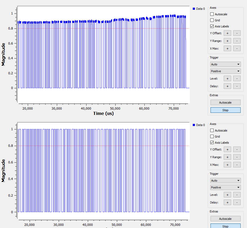
As the initial measurement was over the air (OTA), we have some variability in amplitude however, we can correct for this using the threshold function by defining a 1 V output as every input above 0.8 V and 0 V as every value below 0.1 V on the input to the element. The two magnitude plots show both the raw amplitude data and the amplitude data passed through the threshold function.

Notice in the flow diagram I also decimated the data by seventy and then used the Wave File Sink Element to save the resulting data to a file for processing in the next tool.
Audacity is a free open-source digital audio editor and recording software application. Many people also use it for analyzing demodulated data of many types. It allows you to view and manipulate data down to each sample point. In the following example, I’ve zoomed in enough so that each individual sample point can be seen.

By using the sample edit tool, you can adjust each point, or even change the overall envelope if required. To take the file back into GNU Radio, simply use the Source Wav File Element.
Conclusion
Problems with spurious free dynamic range, images, harmonics and other spurious signals hinder the performance of many SDRs available in the market today, so fundamentally ensuring the acquired data is good before processing is key for successful analysis. Using a high performance RSA306 or RSA500 RTSA as an SDR ensures you acquire high-quality spectrum data. Once you have captured the data, there are many powerful software tools that enable SDR capability.
In this post, I’ve only scratched the surface. Both Octave and GNU Radio, can also be used for clock recover, demodulation and measurements on any type of IQ modulated signals, while Audacity lets you graphically edit at the sample level. Combining high-quality receiver capability with an array of powerful open-source software tools provides almost infinite analysis ability, and the capability to gain deep insight into the radio environment around us. Learn more about spectrum analyzers »